This page was generated from material/1_Using-Jupyter-Lab/1_Using-Jupyter-Lab.ipynb.
Interactive online version:
![]()
Using JuPyteR-Lab
What is jupyter-lab?
jupyter-lab is a browser based editor, with its main focus on editing jupyter-notebooks (which we will also focus on). It is part of the jupyter project, which is an extension of the iPython project. The iPython project and especially the iPython-Notebooks, were developed as an effort to have a free and open source alternative to Mathematica, with a similar interface. This is why it also uses an Input-Output-Cell-Structure and allows you to have your displayed data (i.e.
tables, plots or formulas) right next to the code that produced them.
The name JuPyteR is derived from the programming languages which its development initially was focused on Julia, Python and R. But nowadays it can run a lot more programming languages (i.e. bash, C++ or Fortran), as long as you have the needed interpreter or Compiler installed. For a list of available kernels and how to install them, have a look here.
Why jupyter-notebooks?
jupyter-notebooks are perfect for data exploration and a fast interactive working with code. That you can directly see the output of your code, is helpful if you are new to some specific library or programming in general, because you can see the effect of your changes directly after you applied them. Also since this class is for students and aimed at their day to day university needs (i.e. homework), it is also worth mentioning that jupyter-notebooks can be easily exported to PDF
(File->Export Notebook as...->Export Notebook to PDF).
Note:
If you want develop a library, GUI or similar, you should choose a proper IDE to do so.
How to start jupyter?
To start jupyter-lab simply open a shell/terminal/command line in the folder you want as the base directory for your project and run:
jupyter lab
This will start the jupyter lab server locally and open its url in your default browser.
Note:
You can browse all the subdirectories of that folder in the File Browser but can’t see higher level folders.
Different input modes
Jupyter-lab has two different modes to work with cells the command mode and the insert mode, are used for different interactions with cells.
Command mode
The command mode is used to control the behavior of a whole cell or multiple cells, such as creating, deleting or converting the type of cells. It can also be used to faster scroll your notebook, since the navigation with the arrow keys will be on a cell level. To activate the command mode press Esc. Being in command mode is recognizable by the grayed out interior of the cell, the missing blue border around it and the missing courser.

Most commonly used shortkeys
DD-Deletes currently marked cells (use with caution, this can’t be undone byCtrl+Z)A- Creates a cellAbove the current cellB- Creates a cellBelow the current cellM- Convert current cell to aMarkdown cellY- Convert current cell to aCode cellR- Convert current cell to aRaw cellShift+Arrow Keys- Mark multiple cells
Insert mode
As command mode allows you to interact with cells as a whole, insert mode allows you to change its content.
To activate the insert mode press Enter. Being in insert mode is recognizable by the white interior of the cell, the blue border around it and the blinking courser.

Most commonly used shortkeys
Shift+Enter- Runs/Evaluates the cell and selects the cell below (also works incommand mode)Ctrl+Enter- Runs/Evaluates cell inplace (also works incommand mode)Tab- Autocomplete
Different input cell types
By default cell can have one of three types code cell, markdown cell or raw cell, each serve a different purpose.
Code cells (Ctrl+Y)
The purpose of code cells should be quite self explanatory, these cells are used to write the code you want to execute. Which kind of code you want to execute depends on what you told the cell its content is (see Jupyter-magic), the default being Python or which ever kernel you started the notebook with.
[ ]:
Markdown cells
Markdown cells are used to document your code in a structured and RichText fashion. It allows you to insert headings, lists, tables, images and even videos (for more information ). The special extended kind of Markdown used by jupyter notebooks also allows you to write formulas in LaTeX which are then rendered accordingly.
The expression: $\int^{\infty}_{-\infty} f(x) dx$,
Evaluates to: \(\int^{\infty}_{-\infty} f(x) dx\)
Note:
For the Markdown to be rendered the cell needs to be executed. If a Markdown cell is empty and was executed it will show the boilerplate text:
'Type Markdown and LaTeX: $\alpha^2$'
Raw cells
The purpose of raw cells is to be ignore in the normal notebook and if you convert the notebook i.e. to a LaTeX document, it keeps its content intact and allows you to insert code in your converted document, without having manually temper with the file after conversion over and over again.
Note:
There also are slide cells for presentations, which we might cover in a later chapter.
Jupyter-magic
The so called jupyter-magic is a collection of special commands, which allow you to influence behavior jupyter-lab and/or to run with different kernels. Jupyter-magic is grouped in two kinds, the line-magic and cell magic. An other kind of magic is OSMagic (system calls), which depend on the terminal you opened jupyter-lab with and return the same result as calling that command from the terminal directly.
Note:
On Windows we recommended to run it in Git-Bash or a similar Posix based terminal, since those terminals are much more powerful than the default Windows ones (CMD, Powershell).
Line magic
Commands listed as line magic only apply to a single line and start with a %.
Most commonly used line magic
%lsmagic- Lists the available magic commands.%timeit- This is used to gain information about the execution time of a single line of code, by running it multiple times and measuring the time it took to finish.%ls- Lists all files and directories (OS independent)%pycat <filename>- Displays the content of a file with Python syntax highlighting%matplotlib inline- This is normally used at the start of a notebook and includes figures generated withmatplotlib, which are returned by your code, directly in the corresponding output cell.%matplotlib notebook- More or less the same as%matplotlib inlinebut the plots are more interactive.
[1]:
%lsmagic
[1]:
Available line magics:
%alias  %alias_magic  %autoawait  %autocall  %automagic  %autosave  %bookmark  %cd  %clear  %cls  %colors  %conda  %config  %connect_info  %copy  %ddir  %debug  %dhist  %dirs  %doctest_mode  %echo  %ed  %edit  %env  %gui  %hist  %history  %killbgscripts  %ldir  %less  %load  %load_ext  %loadpy  %logoff  %logon  %logstart  %logstate  %logstop  %ls  %lsmagic  %macro  %magic  %matplotlib  %mkdir  %more  %notebook  %page  %pastebin  %pdb  %pdef  %pdoc  %pfile  %pinfo  %pinfo2  %pip  %popd  %pprint  %precision  %prun  %psearch  %psource  %pushd  %pwd  %pycat  %pylab  %qtconsole  %quickref  %recall  %rehashx  %reload_ext  %ren  %rep  %rerun  %reset  %reset_selective  %rmdir  %run  %save  %sc  %set_env  %store  %sx  %system  %tb  %time  %timeit  %unalias  %unload_ext  %who  %who_ls  %whos  %xdel  %xmode

Available cell magics:
%%!  %%HTML  %%SVG  %%bash  %%capture  %%cmd  %%debug  %%file  %%html  %%javascript  %%js  %%latex  %%markdown  %%perl  %%prun  %%pypy  %%python  %%python2  %%python3  %%ruby  %%script  %%sh  %%svg  %%sx  %%system  %%time  %%timeit  %%writefile

Automagic is ON, % prefix IS NOT needed for line magics.
Cell magic
Commands listed as cell magic apply to a whole cell and start with %%.
Most commonly used cell magic
%%timeit- This is used to gain information about the execution time of a cell of code, by running it multiple times and measuring the time it took to finish.%%bash- Makes the code written in a code cell be executed if it it was a bash script (this also works for other languages, depending on which kernels you have installed).%%writefile <filename>- Writes the content of a cell, to a given file.
[2]:
%%bash
ls -la
total 32
drwxrwxrwx 1 dafuq dafuq  4096 Jul 22 15:54 .
drwxrwxrwx 1 dafuq dafuq  4096 Jun 15 00:15 ..
drwxrwxrwx 1 dafuq dafuq  4096 Feb  7 13:54 .ipynb_checkpoints
-rwxrwxrwx 1 dafuq dafuq 29504 Jul 22 15:55 1_Using-Jupyter-Lab.ipynb
drwxrwxrwx 1 dafuq dafuq  4096 Apr 14 16:19 images
System calls (OSMagics)
System calls start with a ! and execute a command as if it was run in the terminal jupyter lab was started with.
Most commonly used system calls (posix like system)
!ls -la- Lists all files and directories (also hidden ones), as well as their size and read, write, execution rights.!head <filename>- Displays the first lines of a file. This is especially helpful if you want to read text files, which contain a table like structure and you aren’t sure which is the column separating character is.!tail <filename>- Displays the last lines of a file. This is useful if you want to see the progress of a log file (what were the las written entrys).!pwd- Displays the path of the current working directory.
[3]:
!ls -la
total 32
drwxr-xr-x 1 dafuq 197121     0 Jul 22 15:54 .
drwxr-xr-x 1 dafuq 197121     0 Jun 15 00:15 ..
drwxr-xr-x 1 dafuq 197121     0 Feb  7 13:54 .ipynb_checkpoints
-rw-r--r-- 1 dafuq 197121 29504 Jul 22 15:55 1_Using-Jupyter-Lab.ipynb
drwxr-xr-x 1 dafuq 197121     0 Apr 14 16:19 images
Getting familiar with shortcuts (Ctrl+Shift+C)
The easiest way to get familiar with the commands you can run and their keyboard shortcuts, is to use the commands panel (Ctrl+Shift+C or click the Icon ![]() on the left panel selection).
on the left panel selection).
Using commands panel you can also execute commands, which don’t have a shortcut like Restart Kernel and Run All Cells.... Since the search is a fuzzy search it also helps to find commands, which command name you don’t know exactly or to simply look up which commands you can use.
Getting help information
In Python proper written functions/classes/methods contain information about what they are supposed to do and sometimes even usage examples. This is called the docstring and gives the first help in how to use something. In jupyter lab this docstring can be accessed in multiple ways.
Print help (?)
In jupyter lab the ? is a special symbol. If it’s written before or after an expression, the docstring of this expression will be written to the output cell, when the cell is executed.
Note:
If a function/method is being called (has () at the end), this doesn’t work and will give you an error.
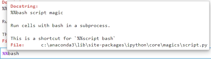
[4]:
%%bash?
Docstring:
%%bash script magic

Run cells with bash in a subprocess.

This is a shortcut for `%%script bash`
File:      c:\anaconda3\lib\site-packages\ipython\core\magics\script.py
[5]:
?%%bash
Docstring:
%%bash script magic

Run cells with bash in a subprocess.

This is a shortcut for `%%script bash`
File:      c:\anaconda3\lib\site-packages\ipython\core\magics\script.py
Quick help (Ctrl+Shift)
Another method to get a fast glimps of the docstring is the quick help function, which is triggered by pressing Ctrl+Shift and will open a small popup window above your cursor. This is especially useful if you just want to look up the function-/method-signature, because you forgot which argument was at which place or you aren’t sure what a keyword argument (kwarg) was called.
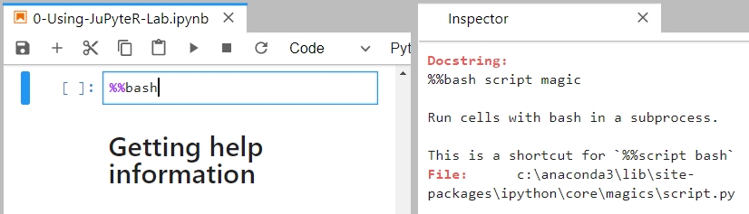
Inspector/Contextual Help window(Ctrl+I)
Last but not least, you can also open the Inspector/Contextual Help window by pressing Ctrl+I. The inspector shows the docstring of the code while you are typing it, in separate tab which you can i.e. arrange right next to your code. This is especially useful if you are learning to program or are starting to work with a new package/library and aren’t familiar with all its functionality yet.
Note:
The Inspector was renamed to Contextual Help in jupyterlab 1.0 and also changed usage behavior. While the Inspector listened to keyboard input and changed its content while typing, with the Contextual Help you select elements by clicking at them and they stay the same while you type.
Cutomizing jupyter-lab
Jupyter lab has a lot of extensions (plugins), which can give you a better experience writing your code and change your editors capabilities how you need them. A list of great extensions can be found at awesome-jupyterlab.
Our recommended extensions are:
Jupyter Widgets Adds sliders and other dynamic inputs you can use to make your notebooks more interactive.
Spellcheckeing Adds spellchecking for english language in markdown cells.
Variableinspector Adds a tab showing the variables which exist in the current session.
Code Formatter Formats your code in the selected style.
Jupyterlab Celltags Allows to add
Tags(meta information) to cells. This addon is part of the jupyter lab core since the 2.0 release.Jupyterlab TOC Adds a TOC (Table of Content) navigation panel.
Jupyterlab Shortcutui Adds a graphical shortcut editor.
Common Pitfalls/Missconceptions
Execution order matters/Interpreter runtime memory
Since normally all cells in jupyter-notebook are executed with the same kernel, the order of execution matters. If you for example define a variable a=2 at the start of a notebook, run some code depending on it (i.e. [In]a+5, [Out] 7) in a different cell, redefine a=3 at the end of your notebook and run the cell with code depending on a again, it will give a different output ([Out] 8) since a has changed. This allows you to run parts of you code without having to
rerun everything again (i.e. very useful if you have a long running simulation and want to style the plot of the results). But it can also lead to problems, when we don’t take this behavior into account when writing the code.
Common Problems:
Broken Notebook - The most severe problem that can occure is that when you open your notebook again and want to run your code (
Run All Cells), it fails at a specific cell telling you that something (i.e. function, variable) isn’t defined. The most common reason for that is that you deleted/renamed that ‘something’/its cell in the last session or defined ‘something’ in a cell below the cell where it is first needed. Since the kernel still remembered/already knew it (deleting from the notebook \(\neq\) deleting from the kernel), everything worked fine, but when you started a new session this ‘something’, wasn’t there when it was needed, since the cells are evaluated in order from top to bottom.
Note:
To solve ordering problems you can move cells in the notebook.
It doesn’t change, even so it should - This is an error, which will lead to a Broken Notebook and often wasts quite some time to find. This mostly happens if you rename (
refacor) a function/variable in one part of your code, but forgot to change it somewhere else, since the kernel remembers the old function/variable, changing the new one won’t affect parts where the old name is still used.
Solution
To make sure that the notebook runs properly even if you run it for the first time, you should always confirm that everything it is runnable with a fresh kernel after refactoring code or before stopping to work on it. You can confirm this by running Restart Kernel and Run All Cells....
Not rendered Plots
By default plots aren’t rendered in the output cells. To activate this for matplotlib (which is also the default backend for pandas) you need to add the magic command %matplotlib inline or %matplotlib notebook.
For other libraries like bokhe or ploty there are special plugins needed to work in jupyter-lab, since they relay on extra javascript code, those plugin are called jupyter extensions.
ModuleNotFoundError
During this course we will introduce different libraries and how to use them. Depending on your Python installation, those might not be installed, which will cause the ModuleNotFoundError when you try to run the examples provided. We recommend to use Anaconda as your installation of choice, since the installer are available for all major platforms (Linux, Windows and MacOS) and most modules come as binaries (called wheels in Python), which means you don’t need to compile them yourself.
Also the default Anaconda installer comes with most libraries we present you included. If any library is still missing you can install it by running:
conda install missing_library_name.
If you don’t want to use Anaconda or this library is only on PyPi (Python Packagagin Index) and not on Anaconda, you can always install it by running:
pip install missing_library_name.
[6]:
import not_a_valid_module
---------------------------------------------------------------------------
ModuleNotFoundError                       Traceback (most recent call last)
<ipython-input-6-b58700dcf11b> in <module>
----> 1 import not_a_valid_module

ModuleNotFoundError: No module named 'not_a_valid_module'